This module's assignment called to explore and visualize social networks, with either NodeXL or R. I am personally biased toward R, and elected to use the "igraph" package with much success. The assignment was overall interesting, and notably, the most difficult part was finding an appropriate and compatible dataset to use.

The concepts of edges and nodes were covered in the reading material, however, it would be useful to learn the process of converting Twitter API data (or other network data) into the edges and nodes used with these types of analysis.

Link to GitHub R Script

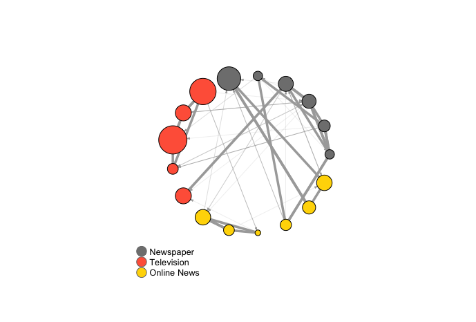
igraph Circle Layout

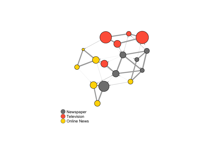
igraph Large Graph Layout

  ############################################################################
  # ------ ------ ------ MOD12: Analyzing Social Networks ------ ------ ------
  ############################################################################
  #' ---
  #' title:   "MOD12: Analyzing Social Networks"
  #' author:  "Kevin Hitt"
  #' date:    "Due: April 12th, 2020"
  #' ---
  #'

  ## Load packages
  library(GGally)
  library(network)
  library(sna)
  library(ggplot2)
  library(igraph)

  ## Example random network visualization
  # generate random graph distribution
  # note: rgraph() [Generate Bernoulli Random Graphs]
  # is a function of the "sna" package
  net <- rgraph(10, mode = "graph", tprob = 0.5)

  # construct network object with "network" package
  net <- network(net, directed = FALSE)

  # add letters as vertex names
  network.vertex.names(net) <- letters[1:10]

  # network visualizations
  ggnet2(net)
  ggnet2(net, node.size = 6, node.color = "black", edge.size = 1, edge.color = "grey")
  ggnet2(net, size = 6, color = rep(c("tomato", "steelblue"), 5))

  # different layout algorithms
  ggnet2(net, size = 6, color = rep(c("tomato", "steelblue"), 5), mode="kamadakawai")
  ggnet2(net, size = 6, color = rep(c("tomato", "steelblue"), 5), mode="target")
  ggnet2(net, size = 6, color = rep(c("gray87", "gray75"), 5), mode="circle",
         label = TRUE, label.alpha = 0.75)


  ## Begin analysis
  # data represents a network of hyperlinks and mentions among news sources
  # Source: https://kateto.net/sunbelt2019.html

  # import data
  nodes <- read.csv("nodes.csv", header=T, as.is=T)
  links <- read.csv("edges.csv", header=T, as.is=T)

  # convert the raw data to an igraph network object
  net <- graph_from_data_frame(d=links, vertices=nodes, directed=T)

  # remove loops from object
  net <- simplify(net, remove.multiple = F, remove.loops = T)

  ## Explore network object
  # view 49 edges of network
  E(net)
  E(net)$type #shows hyperlinks vs. mentions

  # view 17 vertices (nodes) of network
  V(net)
  V(net)$media #shows media source

  # Visualize network object
  # generate colors based on media type:
  colrs <- c("gray50", "tomato", "gold")
  V(net)$color <- colrs[V(net)$media.type]

  # set node size based on audience size value:
  V(net)$size <- V(net)$audience.size*0.6

  # the labels are currently node IDs.
  # setting them to NA will render no labels:
  V(net)$label <- NA

  # set edge width based on weight:
  E(net)$width <- E(net)$weight/6

  # change arrow size and edge color:
  E(net)$arrow.size <- .2
  E(net)$edge.color <- "gray80"

  # set layout to "circle" from igraph package
  graph_attr(net, "layout") <- layout_in_circle

  # plot with legend
  plot(net)
  legend(x=-1.5, y=-1.1, c("Newspaper","Television", "Online News"), pch=21,
         col="#777777", pt.bg=colrs, pt.cex=2, cex=.8, bty="n", ncol=1)

  # plot with "Large Graph Layout" with legend
  graph_attr(net, "layout") <- layout_with_lgl
  plot(net)
  legend(x=-1.5, y=-1.1, c("Newspaper","Television", "Online News"), pch=21,
         col="#777777", pt.bg=colrs, pt.cex=2, cex=.8, bty="n", ncol=1)
          

---